What is Electric Potential & Potential difference?
Table of Contents
- Electric Potential & Potential Difference
- Unit & Dimensions of Electric Potential
- Important Points on Electric Potential & Potential Difference
- Equipotential Surfaces
- Examples based on Electric Potential & Potential Difference
- Potential Energy of a System
- Work Done in an Electric Field
- Motion of a charged particle in an Electric Field
- Example based on motion of a charged particle in an Electric Field

As we know that electric charge forms an electric field around itself. But what if some other charge tries to come into that electric field? Is it that easy to enter into someone’s electric field? The answer is No. As the charge trying to enter also has an electric field. The amount of work needed to move a unit positive charge from one point to another (in the electric field of a charge) is called Electric Potential. The difference of Electric Potential between two points is called Potential difference.
Here you will get to know in detail about:
 Equipotential Surfaces[/caption]
 From Eqn. v = u + at and s = ut + ${1 \over 2}$at² ux = v0 and ax = 0,
ux = v0 = const. and x = v0t
for motion along y-axis as uy = 0 and ay =${{qE} \over m}$,
From Eqn. v = u + at and s = ut + ${1 \over 2}$at² ux = v0 and ax = 0,
ux = v0 = const. and x = v0t
for motion along y-axis as uy = 0 and ay =${{qE} \over m}$,
 ${v_y} = \left[ {{{qE} \over m}} \right]\;t$ and $y = {1 \over 2}\left[ {{{qE} \over m}} \right]\,\;{t^2}$
So, eliminating t between equation for x and y, we have $y = {{qE} \over {2m}}{\left[ {{x \over {{v_0}}}} \right]^2} = {{qE} \over {2mv_0^2}}{x^2}$
If particle is projected perpendicular to field the path is a parabola.
${v_y} = \left[ {{{qE} \over m}} \right]\;t$ and $y = {1 \over 2}\left[ {{{qE} \over m}} \right]\,\;{t^2}$
So, eliminating t between equation for x and y, we have $y = {{qE} \over {2m}}{\left[ {{x \over {{v_0}}}} \right]^2} = {{qE} \over {2mv_0^2}}{x^2}$
If particle is projected perpendicular to field the path is a parabola.
- Electric Potential & Potential difference
- Unit & Dimensions of Electric Potential
- Important Points on Electric Potential & Potential Difference
- Equipotential Surfaces
- Examples based on Electric Potential & Potential Difference
- Potential Energy of a System
- Work Done in an Electric Field
- Motion of a charged particle in an Electric Field
- Example based on motion of a charged particle in an Electric Field
Electric Potential & Potential Difference
An electric potential (also called the electric field potential, potential drop or the electrostatic potential) is the amount of work needed to move a unit of positive charge from a reference point to a specific point inside the field without producing an acceleration. Typically, the reference point is the Earth or a point at infinity. [source] In an electric field, potential at a point is defined as a scalar function of position whose negative gradient at that point gives electric intensity $\mathop E\limits^ \to $ $\mathop E\limits^ \to = - \nabla \,V$ Or $\mathop E\limits^ \to = - grad\,V\,\,or\,\,\mathop E\limits^ \to = - {{dV} \over {dr}}\mathop n\limits^ \to $ So, $dV = - \mathop E\limits^ \to \bullet d\mathop r\limits^ \to $ i.e. $\int_{{V_0}}^V {dV = - } \int_{{r_0}}^r {\mathop E\limits^ \to \bullet \mathop {dr}\limits^ \to } $ or$V - {V_0} = - \int_{{r_0}}^r {\mathop E\limits^ \to \bullet \mathop {dr}\limits^ \to } $ Whenever and wherever possible we take the reference point at infinity and assume the potential to be zero there, so if r0 = ∞, V0 = 0 $V = - \int_\infty ^r {\mathop E\limits^ \to \bullet d\mathop r\limits^ \to } $ or $V = - \int_\infty ^r {{{\mathop F\limits^ \to } \over {{q_0}}} \bullet d\mathop r\limits^ \to } $ $\left[ {as\,\,\mathop E\limits^ \to = {{\mathop F\limits^ \to } \over {{q_0}}}} \right]$ or $V = - {W \over {{q_0}}}$ $\left[ {as\,\,\int {\mathop F\limits^ \to \bullet \mathop {dr}\limits^ \to } = W} \right]$ So potential at a point can be physically interpreted as the negative of the work done by the field in displacing a unit positive charge from some reference point to the given point. Furthermore, as electric field is conservative, so U = –W, $V = {U \over {{q_0}}}$ i.e., U = q0V i.e., potential at a point is numerically equal to the potential energy per unit charge at that point.Unit & Dimensions of Electric Potential
- It is a scalar having dimensions: $V = {W \over {{q_0}}} = {{M{L^2}{T^{ - 2}}} \over {AT}} = M{L^2}{T^{ - 3}}{A^{ - 1}}$ and SI or practical unit is (J/C) called volt (V).
- In CGS system as 1 J = 107 erg and 1 coulomb = 3 × 10⁹ esu of charge = (1/10) emu of charge So, $1V = 1{J \over C} = {{{{10}^7}erg} \over {3 \times {{10}^9}esu\,\,of\,\,ch\arg e}} = {1 \over {300}}esu\,\,of\,\,potential$ and, $1V = 1{J \over C} = {{{{10}^7}erg} \over {(1/10)\,\,emu\,\,of\,\,ch\arg e}} = {10^8}emu\,\,of\,\,potential$
Important Points on Electric Potential & Potential Difference
- As $V = - \int {\mathop E\limits^ \to \bullet \mathop {dr}\limits^ \to } $ so,$E = - {{dV} \over {dr}}$ (a) if E is given, V can be calculated and vice-versa. (b) Negative of the slope of V versus r curve gives electric intensity E.
- If the field is produced by a point charge then, $\mathop E\limits^ \to = {1 \over {4\pi {\varepsilon _0}}}{q \over {{r^3}}}\mathop r\limits^ \to $ and $V = - \int_\infty ^r {\mathop E\limits^ \to \bullet \mathop {dr}\limits^ \to } $ So, $V = - \int_\infty ^r {{1 \over {4\pi {\varepsilon _0}}}} {q \over {{r^3}}}\mathop r\limits^ \to \bullet \mathop {dr}\limits^ \to = - {1 \over {4\pi {\varepsilon _0}}}\int_\infty ^r {{q \over {{r^2}}}dr} $ $V = {1 \over {4\pi {\varepsilon _0}}}{q \over r}$
- For discrete-distribution of charges V = V1 + V2 + V3 + ......... =${1 \over {4\pi {\varepsilon _0}}}\sum {{{q_i}} \over {{r_i}}}$
[caption id="attachment_4321" align="aligncenter" width="364"]
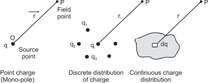 Electric Potential for a) a point charge b) Discrete distribution of charge c) Continuous charge distribution[/caption]
 - For continuous charge distribution, treating the element as point: $dV = {1 \over {4\pi {\varepsilon _0}}}{{dq} \over r}$ , or $V = {1 \over {4\pi {\varepsilon _0}}}\int {{{dq} \over r}} $
- Potential in free space due to a point charge is given by ${V_0} = {1 \over {4\pi {\varepsilon _0}}}{q \over r}$ In a medium of permittivity ε, $V = {1 \over {4\pi \varepsilon }}{q \over r}$ So, ${V \over {{V_0}}} = {{{\varepsilon _0}} \over \varepsilon }$ i.e., $V = {{{V_0}} \over K}$ $\left[ {as{\varepsilon \over {{\varepsilon _0}}} = K} \right]$ i.e., by presence of a medium potential decreases and becomes (1/K) times of its free space value.
- In case of a spherical charge distribution, for external point (r > R), the charge distribution behaves as whole of its charge is concentrated at the center, i.e.,${V_{out}} = {1 \over {4\pi {\varepsilon _0}}}{q \over r}$
[caption id="attachment_4322" align="aligncenter" width="309"]
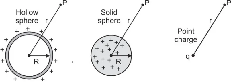 Potential for a Hollow sphere, Solid sphere, Point charge[/caption]
 - In case of spherical charged conductor hollow or solid for an internal point (i.e., r < R), potential everywhere inside is same constant, maximum and equal to its value at the surface, i.e.,
Vin = Vcentre = Vsurface = ${1 \over {4\pi {\varepsilon _0}}}{q \over R}$
[caption id="attachment_4323" align="aligncenter" width="338"]
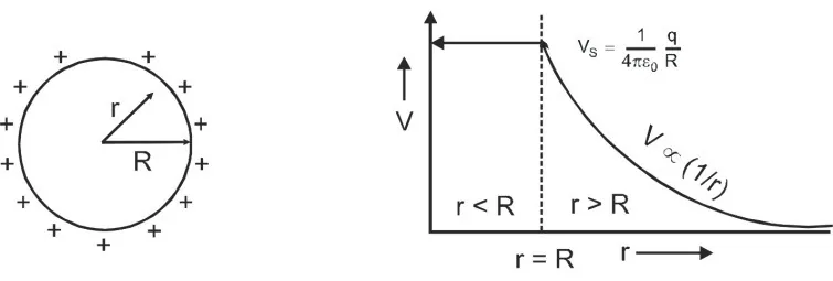 Spherical charged conductor[/caption]
 - In case of spherical volume distribution of charge (e.g., nucleus or uniformly charged dielectric sphere) for an internal point (i.e., r < R) potential varies non-linearly with r as, ${V_{in}} = {1 \over {4\pi {\varepsilon _0}}}{{q\,[3{R^2} - {r^2}]} \over {2{R^3}}}$
[caption id="attachment_4324" align="aligncenter" width="390"]
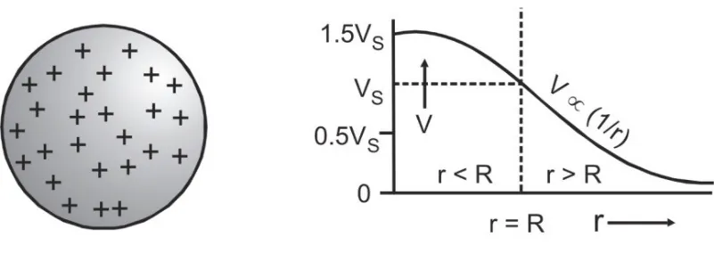 Spherical Volume charge distribution[/caption]
V will be maximum at the center, at r = 0 with ${V_C} = {3 \over 2}\left( {{q \over {4\;\pi \;{\varepsilon _0}\;R}}} \right)$ while at the surface at r = R, VS =${q \over {4\;\pi \;{\varepsilon _0}\;R}}$
so that, ${V_C} = {3 \over 2}{V_S}$
Spherical Volume charge distribution[/caption]
V will be maximum at the center, at r = 0 with ${V_C} = {3 \over 2}\left( {{q \over {4\;\pi \;{\varepsilon _0}\;R}}} \right)$ while at the surface at r = R, VS =${q \over {4\;\pi \;{\varepsilon _0}\;R}}$
so that, ${V_C} = {3 \over 2}{V_S}$ - The electric field is conservative, so work done and hence potential difference between two points is path independent and depends only on the position of points between which the charge is moved. If a charged particle is moved in an electric field between two fixed points A and B whatever be the path, potential difference or work done will be same.
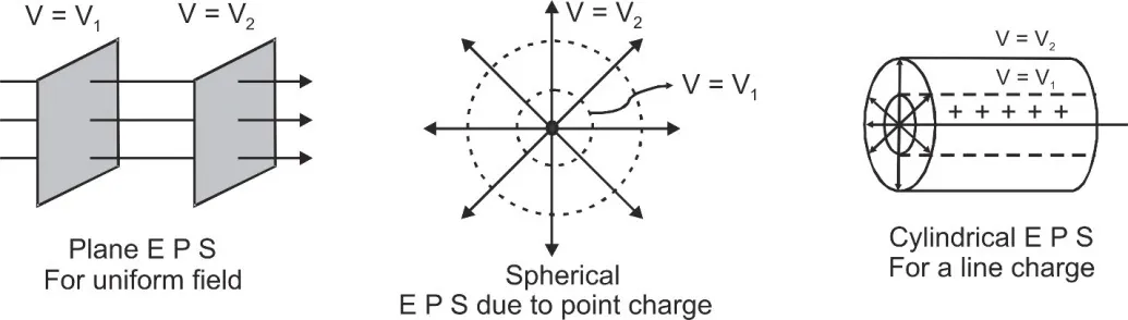
Equipotential Surfaces
For a given charge distribution, locus of all points having same potential is called 'equipotential surface'.Important Points about Equipotential Surfaces:
- Equipotential surfaces can never cross each other otherwise potential at a point will have two values which is not possible.
- Equipotential surfaces are always perpendicular to lines of force.
- If a charge is moved from one point to the other over an equipotential surface, work done will be zero as WAB = – UAB = q(VB – VA) = 0 [as VB = VA]
- The different shapes of equipotential surfaces (EPS) are shown below
Equipotential Surfaces[/caption]
Examples based on Electric Potential & Potential Difference
Q. Infinite number of same charges q are placed at x = 1, 2, 4, 8...... What is the potential at x = 0?
Ans. $V = {1 \over {4\pi {\varepsilon _0}}}\left( {{q \over 1} + {q \over 2} + {q \over 4} + {q \over 8} + ....} \right)$
$ = {q \over {4\pi {\varepsilon _0}}}{1 \over {\left( {1 - {1 \over 2}} \right)}} = {{2q} \over {4\pi {\varepsilon _0}}} = {q \over {2\pi {\varepsilon _0}}}$ [∴ a + ar + .... ∞= r < 1 of r <1]
Q. If the alternative charges are unlike, then what will be the potential?
Ans. Then,$V = {1 \over {4\pi {\varepsilon _0}}}\left[ {{q \over 1} - {q \over 2} + {q \over 4} - {q \over 8} + ......\infty } \right]$
$ = {1 \over {4\pi {\varepsilon _0}}}\left[ {\left( {{q \over 1} + {q \over 4} + .....\infty } \right) - \left( {{q \over 2} + {q \over 8} + .....\infty } \right)} \right]$
$ = {1 \over {4\pi {\varepsilon _0}}}\left[ {{1 \over {1 - {1 \over 4}}} - {1 \over 2}\left( {{1 \over {1 - {1 \over 4}}}} \right)} \right] = {1 \over {4\pi {\varepsilon _0}}}{{2q} \over 3}$ [∴ a + ar + ar² ....... ∞ = ${a \over {1 - r}}$ r < 1]
Q.Electric potential for a point (x, y, z) is given by V = 4x² volt. Electric field at point (1, 0, 2) is-
Ans. $E = - {{dV} \over {dx}}$ = –8x E at (1, 0, 2) = –8V/m
∴ Magnitude of E = 8 V/m and direction is along x-axis.
Q. Electric field is given by $E = {{100} \over {{x^2}}}$. Find potential difference between x = 10 and x = 20 m.
Ans. $E = - {{dV} \over {dx}}$
or dV = – Edx
or $\int_A^B {\;dV} = - \int_A^B {\;E.dx} $
or ${V_B} - {V_A} = - \int_{10}^{20} {} {{100} \over {{x^2}}}dx = - 5$ volt
Potential difference = 5 volt.
Q. Two circular loops of radius 0.05 m and 0.09 m respectively are put such that their axes coincide and their centers are 0.12 m apart. Charge of 10–6 coulomb is spread uniformly on each loop. Find the potential difference between the centers of loops.
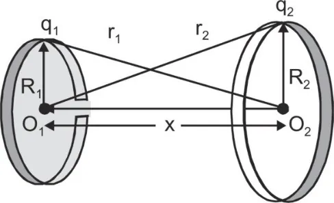
Ans. The potential at the center of a ring will be due to charge on both the rings and as every element of a ring is at a constant distance from the center,
so, ${V_1} = {1 \over {4\pi {\varepsilon _0}}}\left[ {{{{q_1}} \over {{R_1}}} + {{{q_2}} \over {\sqrt {R_2^2 + {x^2}} }}} \right]$
${V_1} = 9 \times {10^9}\left[ {{{{{10}^{ - 4}}} \over 5} + {{{{10}^{ - 4}}} \over {\sqrt {{9^2} + {{12}^2}} }}} \right]$
${V_1} = 9 \times {10^5}\left[ {{1 \over 5} + {1 \over {15}}} \right] = 2.40 \times {10^5}V$
Similarly, ${V_2} = {1 \over {4\pi {\varepsilon _0}}}\left[ {{{{q_2}} \over {{R_2}}} + {{{q_1}} \over {\sqrt {R_1^2 + {x^2}} }}} \right]$
or, ${V_2} = 9 \times {10^5}\left[ {{1 \over 9} + {1 \over {13}}} \right] = {{198} \over {117}} \times {10^5}$ = 1.69 × 10⁵ V
So, V1 – V2 = (2.40 – 1.69) × 105 = 71 kV
Q. A charge Q is distributed over two concentric hollow spheres of radii r and R (> r) such that the surface densities are equal. Find the potential at the common center.
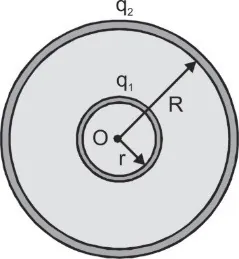
Ans. If q1 and q2 are the charges on spheres of radii r and R respectively, then in accordance with 'conservation of charge' q1 + q2 = Q
According to given problem σ1 = σ2
Or ${{{q_1}} \over {4\pi {r^2}}} = {{{q_2}} \over {4\pi {R^2}}}$
or ${{{q_1}} \over {{q_2}}} = {{{r^2}} \over {{R^2}}}$
So ${q_1} = {{Q{r^2}} \over {({r^2} + {R^2})}}$ and ${q_2} = {{Q{R^2}} \over {({r^2} + {R^2})}}$
Now as potential inside a conducting sphere is equal to its surface, so potential at the common center:$V = {V_1} + {V_2} = {1 \over {4\pi {\varepsilon _0}}}\left[ {{{{q_1}} \over r} + {{{q_2}} \over R}} \right]$
$V = {1 \over {4\pi {\varepsilon _0}}}\left[ {{{Qr} \over {({R^2} + {r^2})}} + {{QR} \over {({R^2} + {r^2})}}} \right] = {1 \over {4\pi {\varepsilon _0}}}{{Q(R + r)} \over {({R^2} + {r^2})}}$
Potential Energy of a System
- The electric potential energy of a system of charges is the work done in bringing these charges from infinity near each other to form the system.
- If a system is given negative of its potential energy, then all charges will move to infinity. This negative value of total energy is called the Binding energy.
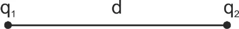
- Energy of a system of two charges $PE = {1 \over {4\pi {\varepsilon _0}}}{{{q_1}{q_2}} \over d}$
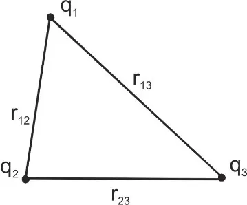
- Energy of a system of three charges PE = ${1 \over {4\pi {\varepsilon _0}}}\left[ {{{{q_1}{q_2}} \over {{r_{12}}}} + {{{q_2}{q_3}} \over {{r_{23}}}} + {{{q_3}{q_1}} \over {{r_{31}}}}} \right]$
- Energy of a system of n charges, PE = \[\frac{1}{2}.\frac{1}{4\pi {{\varepsilon }_{0}}}\sum\limits_{i=1}^{n}{{}}\sum\limits_{\begin{smallmatrix}j=1 \\i\,\ne\end{smallmatrix}}^{n}{\,\,\frac{{{q}_{i\,\,}}{{q}_{j}}}{{{r}_{ij}}}}\]
Work Done in an Electric Field
- If electric potential at a point is V then potential energy of a charge placed at that point will be qV.
- Work done in moving a charge from A to B is equal to change in PE of that charge WAB = work done from A to B = PEB – PEA = q (VB – VA)
- Work done in moving a charge along a closed path in an electric field is zero.
- Total energy remains constant in an electric field i.e. KEA + PEA = KEB + PEB KE = Kinetic Energy PE = Potential Energy
- A free charge moves from higher PE to lower PE state in an electric field. (i) A positive charge moves from higher potential to lower potential (ii) a negative charge moves from lower potential to higher potential (iii) Work done in displacement of a charge through $\mathop r\limits^ \to $ by a force $\mathop F\limits^ \to \,\,\,is\,\,W = \mathop F\limits^ \to .\mathop r\limits^ \to $
Motion of a charged particle in an Electric Field
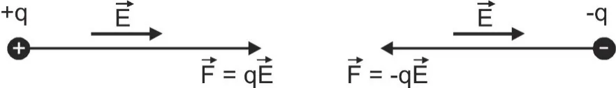
In case of motion of a charged particle in an electric field:- A point charge experiences a force whether it is at rest or in motion $\mathop F\limits^ \to = q\mathop E\limits^ \to $.
- The direction of force is parallel to the field if the charge is positive and opposite to the field if charge is negative.
- Electric field is conservative so work done is independent of path and work done in moving a point charge q between two fixed points having a potential difference V is equal to, WAB = – UAB = q(VB – VA) = qV
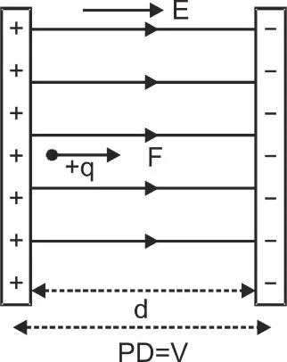
- Work is done in moving a charged particle in an electric field unless the points are at same potential
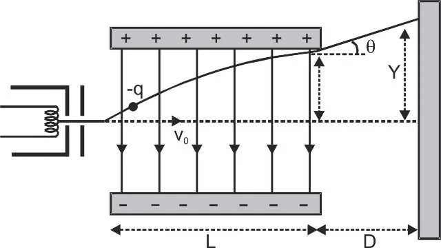
[caption id="attachment_4331" align="aligncenter" width="351"]
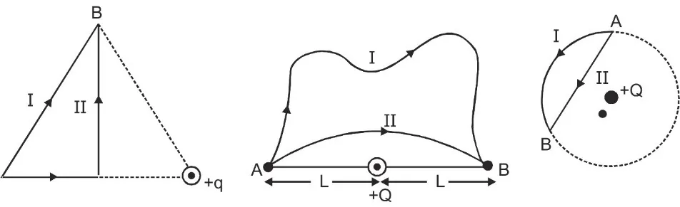 Work is done in moving a charged particle in an electric field[/caption]
 - When a charged particle is accelerated by a uniform or non-uniform electric field then by work energy theorem ΔKE = W, So, ${1 \over 2}m{v^2} - {1 \over 2}m{u^2} = qV$ or final velocity $v = \sqrt {\left[ {{u^2} + {{2qV} \over m}} \right]} $ If the charged particle is initially at rest, then $v = \sqrt {{{2qV} \over m}} $ . If the field is uniform, E = (V/d) so $v = \sqrt {{{2qEd} \over m}} $
- In motion of a charged particle in a uniform electric field if force of gravity does not exist or is balanced by some other force say reaction or neglected then $\mathop a\limits^ \to = {{\mathop F\limits^ \to } \over m} = {{\mathop {qE}\limits^ \to } \over m} = cons\tan t$ [as $\mathop F\limits^ \to = \mathop {qE}\limits^ \to $] Here equations of motion are valid.
From Eqn. v = u + at and s = ut + ${1 \over 2}$at² ux = v0 and ax = 0,
ux = v0 = const. and x = v0t
for motion along y-axis as uy = 0 and ay =${{qE} \over m}$,
${v_y} = \left[ {{{qE} \over m}} \right]\;t$ and $y = {1 \over 2}\left[ {{{qE} \over m}} \right]\,\;{t^2}$
So, eliminating t between equation for x and y, we have $y = {{qE} \over {2m}}{\left[ {{x \over {{v_0}}}} \right]^2} = {{qE} \over {2mv_0^2}}{x^2}$
If particle is projected perpendicular to field the path is a parabola.
Example based on motion of a charged particle in an Electric Field
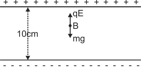
Q. An oil drop 'B' has charge 1.6 × 10⁻¹⁹ C and mass 1.6 × 10⁻¹⁴ kg. If the drop is in equilibrium position, then what will be the potential diff. between the plates. [The distance between the plates is 10mm]
Ans. For equilibrium, electric force = weight of drop
⇒ qE = mg or $q.{V \over d} = mg$
⇒ $V = {{mgd} \over q}$ = 1.6 × 10–14 × 9.8 × 10 × 10–3 / 1.6 × 10–19 = 104 V